In WPS Office Spreadsheet, you can automatically fill a column with serial numbers such as 1, 2, 3, 4, 5, 6, 7… without typing each number manually. There are several methods, but the easiest is to use the Fill Handle or a formula.

Method 1: Use the Fill Handle (Easiest Method)

Follow these steps:

1. Open your spreadsheet in WPS Office.
2. Click the first cell where you want the serial numbers to begin, for example, A2.
3. Type 1 and press Enter.
4. In the cell below it, A3, type 2 and press Enter.
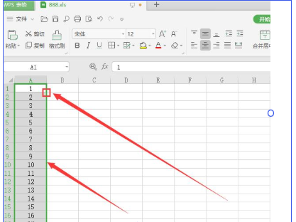
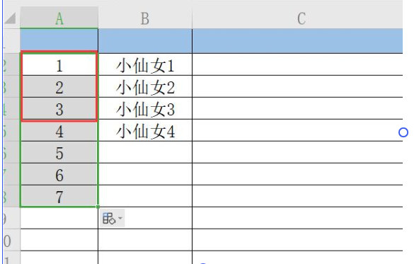
5. Select both cells, A2 and A3, by dragging across them or clicking A2 and holding Shift while clicking A3.
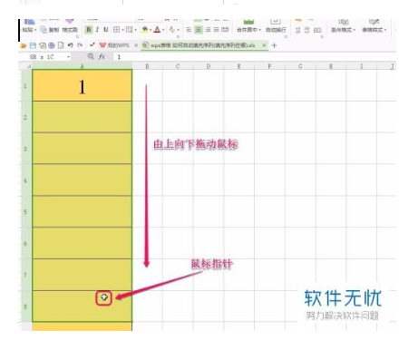
6. Move your mouse to the small square at the bottom-right corner of the selected cells. This is called the Fill Handle.
7. When the cursor changes to a small black cross, click and drag it downward to the last row you need.

WPS will continue the sequence automatically:

Cell	Serial number
A2	1
A3	2
A4	3
A5	4
A6	5
A7	6
A8	7
A9	8
A10	9
A11	10

Important: Enter both 1 and 2 before dragging. If you enter only 1, WPS may copy the number 1 into every selected cell instead of creating a sequence.

Method 2: Use a Formula to Generate Serial Numbers Automatically

This method is useful when you have a long list and want the serial numbers to calculate automatically.

Suppose your serial numbers will be in column A, starting from cell A2.

1. Click cell A2.
2. Enter this formula:

=ROW()-1

3. Press Enter.
4. Click A2 again and drag the Fill Handle downward to the desired row.

The formula will generate serial numbers automatically:

• A2 = 1
• A3 = 2
• A4 = 3
• A5 = 4
• A6 = 5

The formula works because ROW() returns the row number of the cell containing the formula. Subtracting 1 makes the numbering start at 1 in row 2.

If your serial numbers start in row 5, use =ROW()-4 in cell A5.

Alternative formula for numbering only rows containing data

Suppose column B contains names, product descriptions, or other records, and you want column A to display a serial number only when column B is not empty.

Enter this formula in A2:

=IF(B2="","",COUNTA($B$2:B2))

Then drag it downward.

This formula leaves the serial-number cell blank when the corresponding cell in column B is empty. When column B contains a value, the formula displays a serial number.

For example:

A — S/N	B — Name
1	John
2	Mary
3	Peter
4	Grace

The numbering follows the number of non-empty cells above and including the current row.

Method 3: Use the Fill Series Command

If you want to generate hundreds or thousands of serial numbers, the Fill Series command can save time.

1. Type 1 in cell A2.
2. Select the range you want to number, such as A2:A101, for 100 serial numbers.
3. Go to the Home tab.
4. Look for Fill in the editing tools. Depending on your WPS version, it may appear under a menu or dropdown.
5. Select Series or Fill Series.
6. Set the following values:
   • Series in: Columns
   • Type: Linear
   • Step value: 1
   • Stop value: 100, if required
7. Click OK.

WPS will fill the selected cells with consecutive numbers.

Which Method Should You Use?

Method	Best use
Fill Handle	Quickly numbering a short or medium list
=ROW()-1	Generating serial numbers using formulas
=IF(B2="","",COUNTA($B$2:B2))	Numbering only rows containing data
Fill Series	Filling a large, predefined range

My recommendation: If you simply want to number rows from 1 to 100 or more in WPS Spreadsheet, type 1 in A2 and 2 in A3, select both cells, and drag the Fill Handle down. It is the simplest method and requires no formula.